Cancer by County
Goal
Complete this online challenge and try to predict cancer mortality rates for US counties with linear regression.
Data Collection
Downloaded via the above link, feature descriptions are there as well.
Data Engineering
Some of the features are immediately show signs of incorrectly entered values:
Median Age
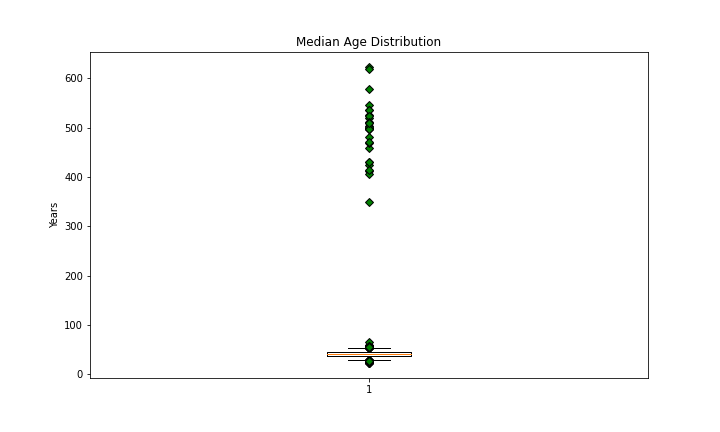
countyData['MedianAge'].describe()
count    3047.000000
mean       45.272333
std        45.304480
min        22.300000
25%        37.700000
50%        41.000000
75%        44.000000
max       624.000000
Given the values of the outliers I think it’s likely that these inputs have months as their unit.
print(countyData[countyData['MedianAge'] < 100]['MedianAge'].max())
print(countyData[countyData['MedianAge'] < 100]['MedianAge'].min())
print(countyData[countyData['MedianAge'] > 100]['MedianAge'].max()/12)
print(countyData[countyData['MedianAge'] > 100]['MedianAge'].min()/12)

65.3
22.3
52.0
29.1
The outliers when divided by 12 are within the range of ‘normal’ inputs:
countyData.loc[countyData['MedianAge'] > 100, ['MedianAge']] = countyData.loc[countyData['MedianAge'] > 100]['MedianAge']/12
Average Household Size
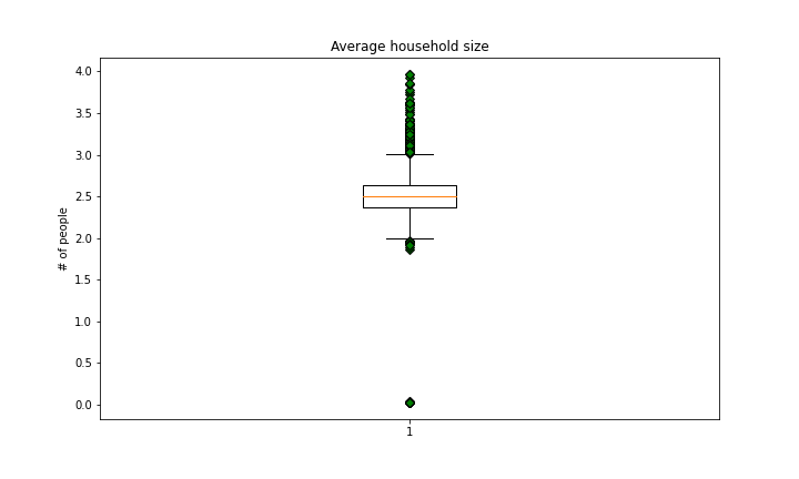
There are a number of outliers here.
countyData[countyData['AvgHouseholdSize'] < 1]['AvgHouseholdSize']

23      0.0263
33      0.0280
121     0.0225
122     0.0242
196     0.0243
         ...
2735    0.0270
2768    0.0260
2856    0.0270
Multiplying by 100 would put all of these values within the inner 2 quartiles of the distribution so I applied that transformation:
countyData.loc[countyData['AvgHouseholdSize'] < 1,['AvgHouseholdSize']] = countyData[countyData['AvgHouseholdSize'] < 1]['AvgHouseholdSize']*100
avgDeathsPerYear & popEst2015
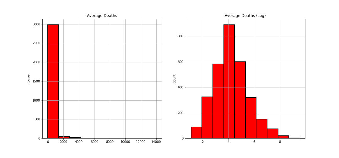
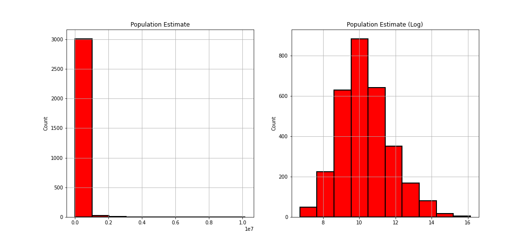
Both of these were showing heavily right skewed distributions so I applied a logarithmic transformation to normalize it:
countyData['avgDeathsPerYear'] = np.log(countyData['avgDeathsPerYear'])
countyData['popEst2015'] = np.log(countyData['popEst2015'])
Features Dropped
binnedInc column was dropped because it is a categorical feature that doesn’t provide any information that medianIncome doesn’t.
Geography was dropped as short of adding geographical coordinates there’s no information to be obtained here.
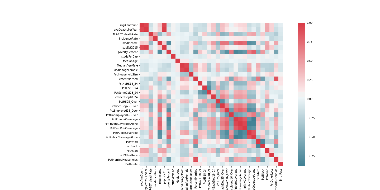
'avgAnnCount', 'PercentMarried', 'povertyPercent' were also dropped as they were highly correlated with other features:
countyData = countyData.drop(columns=['binnedInc', 'Geography'])
Missing Data
To check for NaN values and list columns with such values:
nan_values = countyData.isna()
nan_columns = nan_values.any()
columns_with_nan = countyData.columns[nan_columns].tolist()
print(columns_with_nan)
Replaced any NaNs with the median value of the column:
median = countyData['PctSomeCol18_24'].median()
countyData['PctSomeCol18_24'].fillna(median, inplace=True)

median = countyData['PctEmployed16_Over'].median()
countyData['PctEmployed16_Over'].fillna(median, inplace=True)

median = countyData['PctPrivateCoverageAlone'].median()
countyData['PctPrivateCoverageAlone'].fillna(median, inplace=True)
Feature Scaling
Applied mean normalization:
countyData=(countyData-countyData.mean())/countyData.std()
Results
Training and validation score reflect the R2, Coefficient of determination, of the between the features and the target variable. The closer to 1 the more the features explain the target. The RMSE is how far the predictions are off on average.
Baseline (none of the above applied):
Training Score: 0.52
Validation Score: 0.51
RMSE = 19.68
With Data Cleaning:
Training Score: 0.79
Validation Score: 0.76
RMSE = 12.28
Code
Libraries:
import pandas as pd
import numpy as np
import matplotlib.pyplot as plt
import math
from scipy import stats
from sklearn.linear_model import LinearRegression
from sklearn.pipeline import make_pipeline
from sklearn.metrics import mean_squared_error
from sklearn.model_selection import train_test_split
from sklearn.preprocessing import PolynomialFeatures
import seaborn as sns
from statsmodels.nonparametric.smoothers_lowess import lowess
Data Engineering:
countyData = pd.read_csv('cancer_reg.csv', encoding='latin-1')
target = countyData['TARGET_deathRate']
countyData = countyData.drop(columns=['TARGET_deathRate', 'binnedInc', 'Geography','PercentMarried', 'povertyPercent'])
countyData.loc[countyData['MedianAge'] > 100, ['MedianAge']] = countyData.loc[countyData['MedianAge'] > 100]['MedianAge']/12
countyData.loc[countyData['AvgHouseholdSize'] < 1,['AvgHouseholdSize']] = countyData[countyData['AvgHouseholdSize'] < 1]['AvgHouseholdSize']*100

countyData['avgAnnCount'] = np.log(countyData['avgAnnCount'])
countyData['avgDeathsPerYear'] = np.log(countyData['avgDeathsPerYear'])
countyData['popEst2015'] = np.log(countyData['popEst2015'])

median = countyData['PctSomeCol18_24'].median()
countyData['PctSomeCol18_24'].fillna(median, inplace=True)

median = countyData['PctEmployed16_Over'].median()
countyData['PctEmployed16_Over'].fillna(median, inplace=True)

median = countyData['PctPrivateCoverageAlone'].median()
countyData['PctPrivateCoverageAlone'].fillna(median, inplace=True)

countyData=(countyData-countyData.mean())/countyData.std()
Model:
trainingScore = 0
validationScore = 0
for i in range(0,500):
    X_train, X_valid, y_train, y_valid = train_test_split(countyData, target, test_size=0.2)
    model = make_pipeline(
        LinearRegression()
    )
    model.fit(X_train, y_train.values)
    trainingScore += model.score(X_train, y_train)
    validationScore += model.score(X_valid, y_valid)
print(trainingScore/500)
print(validationScore/500)
y_predicted = model.predict(X_valid)
regression_model_mse = mean_squared_error(y_predicted, y_valid)
print(math.sqrt(regression_model_mse))